逻辑斯特回归 (Case Study)

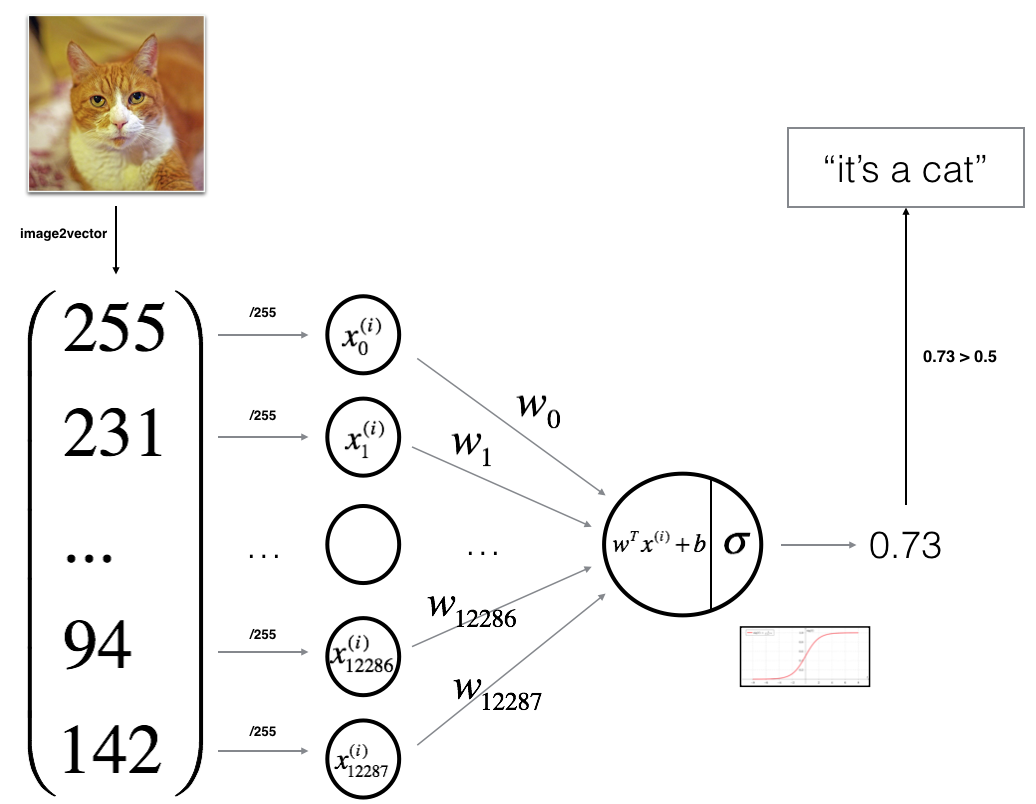
task: 训练一个识别猫的LR

输入数据的预处理:
- Shape and Dimension 明确训练集/测试集数据的形状和维度，比如数量和样本特征维度 (m_train, m_test, num_px, ...)
- Reshape 输入数据shape 使其成为一个合理输入 (num_px * num_px * 3, 1)
- "Standardize" 数据归一化处理

1 - 模型(Model)

训练一个识别图片是否是猫的LR。一个简单的二分类器，直接使用 sigmoid 做输出层。Logistic Regression 就是一个简单的 Neural Network!

模型的数学公式:

对某个输入数据 $x^{(i)}$, 下面是公式

$$z^{(i)} = w^T x^{(i)} + b \tag{1}$$
$$\hat{y}^{(i)} = a^{(i)} = sigmoid(z^{(i)})\tag{2}$$

2 - 损失/策略(Cost)

二分类器可以直接使用 cross-entropy 交叉熵来定义损失函数:
$$ \mathcal{L}(a^{(i)}, y^{(i)}) = - y^{(i)} \log(a^{(i)}) - (1-y^{(i)} ) \log(1-a^{(i)})\tag{3}$$
$$ J = \frac{1}{m} \sum_{i=1}^m \mathcal{L}(a^{(i)}, y^{(i)})\tag{6}$$

3 - 优化/学习算法(Algorithm)

构建神经网络的基本步骤:
1. 定义模型架构
2. 初始化模型参数
3. Loop:
- 前向传播计算损失 (forward propagation)
- 反向传播计算梯度 (backward propagation)
- 使用梯度更新参数 (gradient descent)基本上全部是梯度下降法，还有牛顿法

3.1 - Forward and Backward propagation

Forward Propagation:
- 输入X
- 计算激活 $A = \sigma(w^T X + b) = (a^{(0)}, a^{(1)}, ..., a^{(m-1)}, a^{(m)})$
- 计算损失: $J = -\frac{1}{m}\sum_{i=1}^{m}y^{(i)}\log(a^{(i)})+(1-y^{(i)})\log(1-a^{(i)})$

简单的求导公式即 Backward Propagation:

$$ \frac{\partial J}{\partial w} = \frac{1}{m}X(A-Y)^T\tag{7}$$
$$ \frac{\partial J}{\partial b} = \frac{1}{m} \sum_{i=1}^m (a^{(i)}-y^{(i)})\tag{8}$$

def propagate(w, b, X, Y):

    m = X.shape[1]

    # FORWARD PROPAGATION (FROM X TO COST)
    A = sigmoid(np.dot(w.T, X) + b)              # compute activation
    cost = (-1. / m) * np.sum((Y*np.log(A) + (1 - Y)*np.log(1-A)), axis=1)     # compute cost

    # BACKWARD PROPAGATION (TO FIND GRAD)
    dw = (1./m)*np.dot(X,((A-Y).T))
    db = (1./m)*np.sum(A-Y, axis=1)

    assert(dw.shape == w.shape)
    assert(db.dtype == float)
    cost = np.squeeze(cost)
    assert(cost.shape == ())

    grads = {"dw": dw,
             "db": db}

    return grads, cost

3.2 优化算法

优化过程就是通过最小化损失函数 $J$ 来学习参数 $w$ and $b$. 对参数 $\theta$, 优化规则是 $ \theta = \theta - \alpha \text{ } d\theta$, $\alpha$ 为学习速率 learning_rate.

def optimize(w, b, X, Y, num_iterations, learning_rate, print_cost = False):

    costs = []

    for i in range(num_iterations):


        # Cost and gradient calculation
        grads, cost = propagate(w=w, b=b, X=X, Y=Y)

        # Retrieve derivatives from grads
        dw = grads["dw"]
        db = grads["db"]

        # update rule
        w = w - learning_rate*dw
        b = b -  learning_rate*db

        # Record the costs
        if i % 100 == 0:
            costs.append(cost)

        # Print the cost every 100 training examples
        if print_cost and i % 100 == 0:
            print ("Cost after iteration %i: %f" %(i, cost))

    params = {"w": w,
              "b": b}

    grads = {"dw": dw,
             "db": db}

    return params, grads, costs

浅层神经网络(Shallow Neural Net)

1 - 模型 Neural Network model

神经网络中的一个隐藏层节点其实是一个逻辑斯特回归分类器。

model:

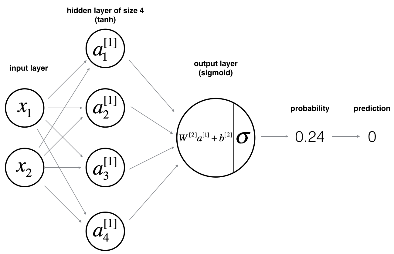
单隐藏层的神经网络可以看成是以逻辑斯特回归为基础神经节点, 再多加一层再次向前传播而已. 隐藏层的每一个单元就可以看成是一个逻辑斯特回归,

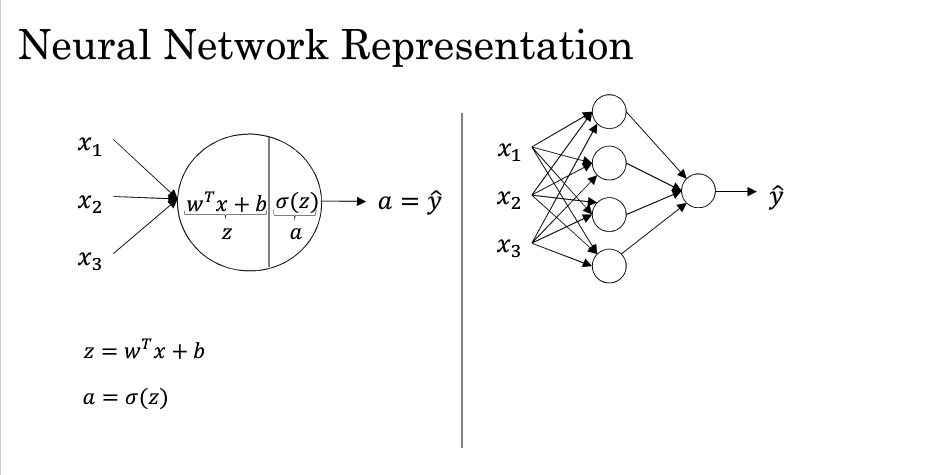
你可以把每个隐藏层节点都是一个逻辑斯特回归.

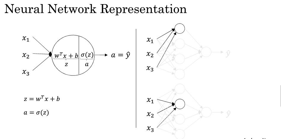
下面用公式来表示一个前向传播的过程:

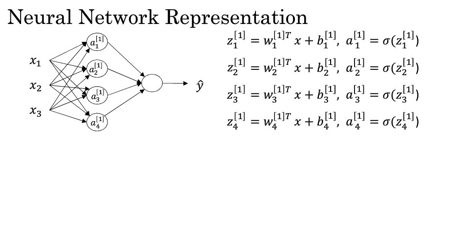
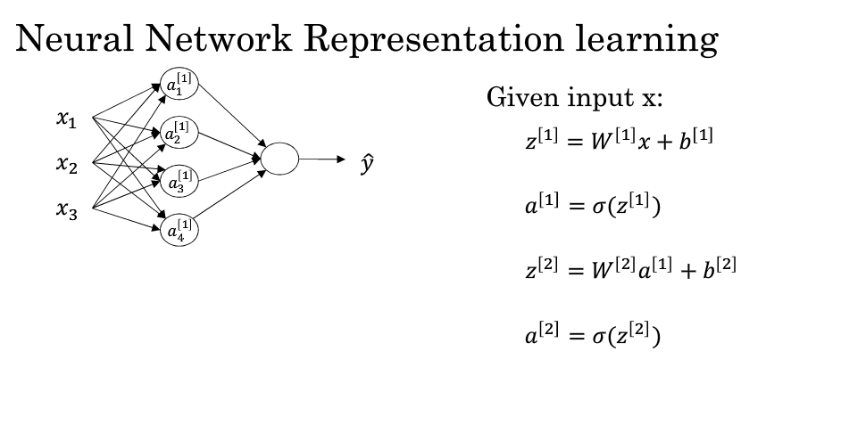
整体架构：

Mathematically:

$$z^{[1] (i)} = W^{[1]} x^{(i)} + b^{[1] (i)}\tag{1}$$
$$a^{[1] (i)} = \tanh(z^{[1] (i)})\tag{2}$$
$$z^{[2] (i)} = W^{[2]} a^{[1] (i)} + b^{[2] (i)}\tag{3}$$
$$\hat{y}^{(i)} = a^{[2] (i)} = \sigma(z^{ [2] (i)})\tag{4}$$

$$
\begin{align}
y^{(i)}_{prediction} =
\begin{cases}
1 & \mbox{if } a^{[2] (i)} > 0.5 \\
0 & \mbox{otherwise }
\end{cases}
\end{align}\tag{5}
$$

2 - 损失/策略

$$
J = - \frac{1}{m} \sum\limits_{i = 0}^{m} \large\left(\small y^{(i)}\log\left(a^{[2] (i)}\right) + (1-y^{(i)})\log\left(1- a^{[2] (i)}\right) \large \right) \small \tag{6}
$$

3 - 学习/优化算法

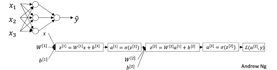
3.1 Forward and Backward Propagation

反向传播，使用链式法则和微分进行求导得到。这里关于向量求导和标量相比，最难的部分是 shape 和导数形式问题。求导规则和标量一样，但是需要注意点乘和转置，以及求和形式。这里有一个Trick是根据 dW 的shape 和 dimension 来推断出导数公式。

举个列子, 以下是 sigmoid 作为输出层构成的二分类器的交叉熵损失函数的向量形式, 改公式是 (6) 的向量形式：
$$
L = -\frac{1}{m}{Y\log(A)+ (1-Y)\log(1-A)} \qquad (7)
$$

$$
A
=
\begin{bmatrix}
a_1 \\
a_2 \\
\vdots \\
a_t \\
\vdots \
a_m
\end{bmatrix} \quad
Y
=
\begin{bmatrix}
y_1 & y_2 & \cdots & y_t & \cdots y_m
\end{bmatrix}
$$
对 A 向量中的每个元素求导

$$
d_a
=
\begin{bmatrix}
d_{a_1} \\
d_{a_2} \\
\vdots \\
d_{a_t} \\
\vdots \\
d_{a_m}
\end{bmatrix}
=
\begin{bmatrix}
-\frac{1}{m}(\frac{y_1}{a_1}-\frac{1-y_1}{1-a_1}) \\
-\frac{1}{m}(\frac{y_2}{a_2}-\frac{1-y_2}{1-a_2}) \\
\vdots \\
-\frac{1}{m}(\frac{y_t}{a_t}-\frac{1-y_t}{1-a_t}) \\
\vdots \\
-\frac{1}{m}(\frac{y_m}{a_m}-\frac{1-y_m}{1-a_m})
\end{bmatrix}
$$

以上的标量形式累积成一个向量写法之后，就是以下公式：

$$
\begin{align}
d_{a^{L}} &= \frac{\partial L}{\partial A} & \\
&= -\frac{1}{m}(\frac{Y^T}{A}-\frac{1-Y^T}{1-A}) & \\
&= \frac{1}{m}{\frac{A-Y^T}{A*(1-A)}} \qquad (3)
\end{align}
$$

其中的 $A * (1-A)$ 以及 $(A-Y^T) / A * (1-A)$ 中的 * /都是element-wise 的矩阵运算;

$$
\begin{align}
d_{z^{L}} &= \frac{\partial L}{\partial A}\frac{\partial A}{\partial Z} & \\
&= d_{a}A*(1-A) & \\
&= \frac{1}{m}(A-Y^T) \qquad (4)
\end{align}
$$

消除后可以化简, 这里的 A 是最后一层的激活输出;

$$
\begin{align}
d_{w^{L}} &= \frac{\partial L}{\partial Z}\frac{\partial Z}{\partial W} & \\
&= d_{z^{L}}(A^{L-1})^T \qquad (5)
\end{align}
$$

为了保持得到的导数矩阵的维度和$W$ 保持一致,我们必须对链式法则求导的结果运算进行转置和交换,来保证维度的一致性; 上式中 $\frac{\partial Z}{\partial W}$ 得到 $A^{L-1}$, $\frac{\partial L}{\partial Z}$ 得到 $d_z$, 由于 $d_w$ 的维度应该是 $(n_{L}, n_{L-1})$, 而 $d_z$ 的维度是 $(n_{L}, m)$, $A^{L-1}$ 的维度是 $(n_{L-1}, m)$, 因此我们推断出 $d_w = d_{z^{L}}(A^{L-1})^T$ 才合理。

最后，偏移量的导数形式很奇怪，会多出一个求和。原因是 b（如果是scalar）的系数可以看成是全一的矩阵[[1,1,1,...1]],其系数在累计 m 个例子的误差的时候，被求和了，因此会出现求和公式。比如 $b^{L}$ 的系数shape 是 $(n_{L}, 1)$, 而在求Z的时候，b会被广播成 $(n_L, m)$, 然后计算损失的时候会在m维度上累加m次，因此出现了累加 m次。如果无法理解，可以直接记住这个公式。反向传播都一样。

$$
\begin{align}
d_{b^{L}} &= \frac{\partial L}{\partial Z}\frac{\partial Z}{\partial b} & \\
&= \sum\limits_{i = 0}^{m}{d_{z^{L}}} \qquad (5)
\end{align}
$$

def backward_propagation(parameters, cache, X, Y):
    m = X.shape[1]

    # First, retrieve W1 and W2 from the dictionary "parameters".
    W1 = parameters["W1"]
    W2 = parameters["W2"]

    # Retrieve also A1 and A2 from dictionary "cache".
    A1 = cache["A1"]
    A2 = cache["A2"]

    # Backward propagation: calculate dW1, db1, dW2, db2. 
    dZ2= A2 - Y
    dW2 = (1/m) * np.dot(dZ2, A1.T)
    db2 = (1/m) * np.sum(dZ2, axis=1, keepdims=True)
    dZ1 = np.multiply(np.dot(W2.T, dZ2), (1 - np.power(A1, 2)))
    dW1 = (1/m) * np.dot(dZ1, X.T)
    db1 = (1/m) * np.sum(dZ1, axis=1, keepdims=True)

    grads = {"dW1": dW1,
             "db1": db1,
             "dW2": dW2,
             "db2": db2}

    return grads

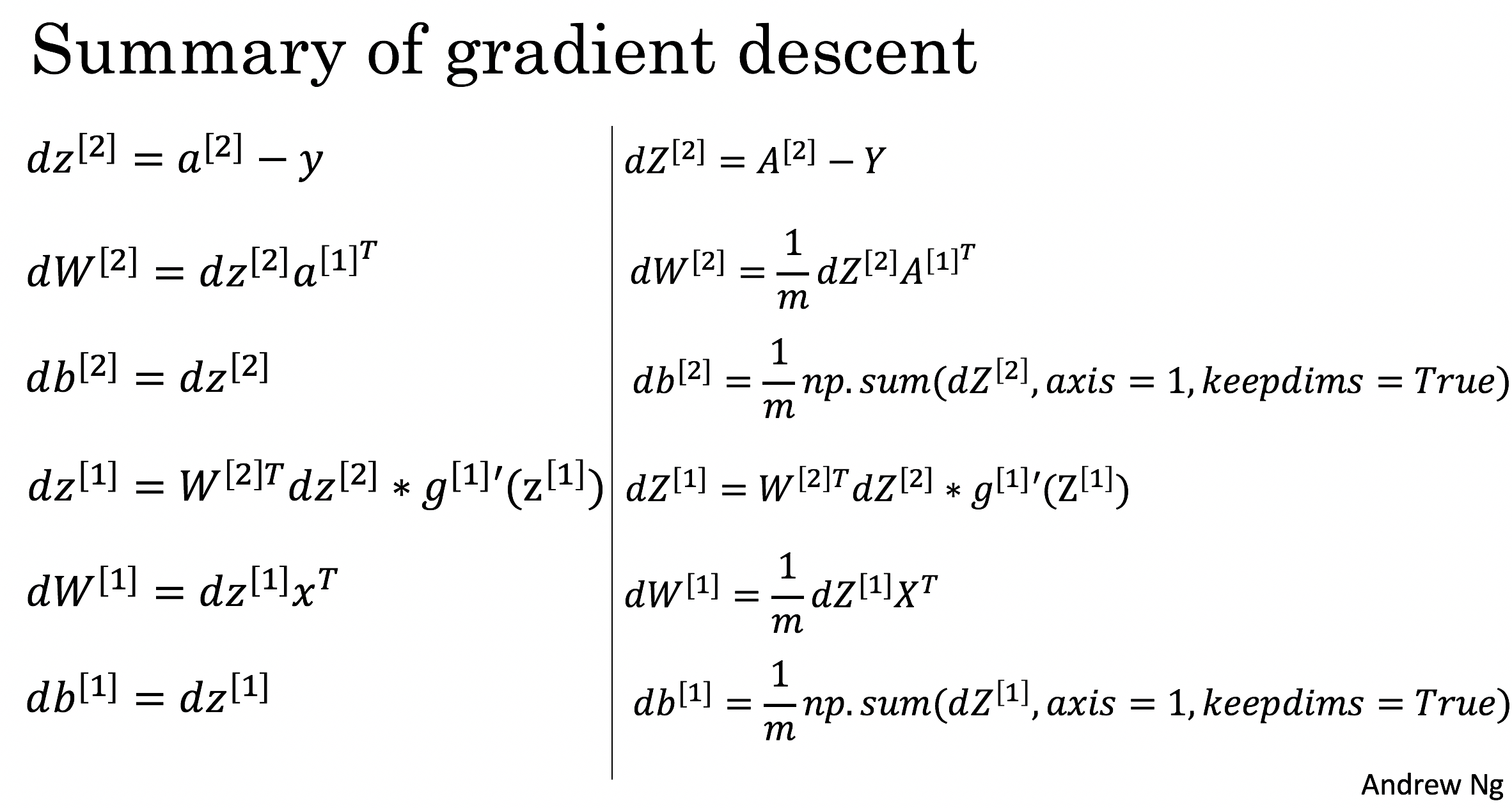
3.2 参数更新公式

$\frac{\partial \mathcal{J} }{ \partial z_{2}^{(i)} } = \frac{1}{m}(a^{[2] (i)} - y^{(i)}) $

$\frac{\partial \mathcal{J} }{ \partial W_2 } = \frac{\partial \mathcal{J} }{ \partial z_{2}^{(i)} } a^{[1] (i) T} $

$\frac{\partial \mathcal{J} }{ \partial b_2 } = \sum_i{\frac{\partial \mathcal{J} }{ \partial z_{2}^{(i)}}} $

$\frac{\partial \mathcal{J} }{ \partial z_{1}^{(i)} } = W_2^T \frac{\partial \mathcal{J} }{ \partial z_{2}^{(i)} } * ( 1 - a^{[1] (i) 2})$

$\frac{\partial \mathcal{J} }{ \partial W_1 } = \frac{\partial \mathcal{J} }{ \partial z_{1}^{(i)} } X^T $

$\frac{\partial \mathcal{J} }{ \partial b_1 } = \sum_i{\frac{\partial \mathcal{J} }{ \partial z_{1}^{(i)}}} $

符号 $*$ 表示 elementwise 乘积.
偏导和微分等价:
- $dW1 = \frac{\partial \mathcal{J} }{ \partial W_1 }$
- $db1 = \frac{\partial \mathcal{J} }{ \partial b_1 }$
- $dW2 = \frac{\partial \mathcal{J} }{ \partial W_2 }$
- $db2 = \frac{\partial \mathcal{J} }{ \partial b_2 }$

参数更新，mini-BGD
- $W2 = W2 - \lambda * dW2$
- $b2 = b2 - \lambda * db2$
- $W1 = W1 - \lambda * dW1$
- $b1 = b1 - \lambda * db1$

def update_parameters(parameters, grads, learning_rate = 1.2):
    # Retrieve each parameter from the dictionary "parameters"
    W1 = parameters["W1"]
    b1 = parameters["b1"]
    W2 = parameters["W2"]
    b2 = parameters["b2"]

    # Retrieve each gradient from the dictionary "grads"
    dW1 = grads["dW1"]
    db1 = grads["db1"]
    dW2 = grads["dW2"]
    db2 = grads["db2"]

    # Update rule for each parameter
    W1 = W1 - learning_rate * dW1
    b1 = b1 - learning_rate * db1
    W2 = W2 - learning_rate * dW2
    b2 = b2 - learning_rate * db2

    parameters = {"W1": W1,
                  "b1": b1,
                  "W2": W2,
                  "b2": b2}

    return parameters

SoftMax 多分类

1- softmax activation

softmax函数是机器学习中多分类问题最常用的函数之一，他是一种概率估计，可以用概率来解释多分类的数值。对于神经网络中的最后一层输出层，激活函数可以采用softmax。

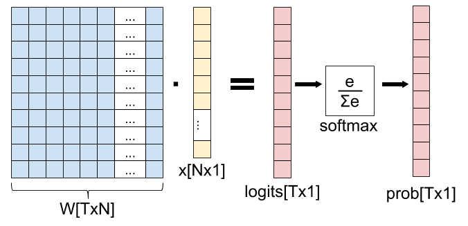
$$
a^{L}_{j} = \frac{e^{z^{L}_j}}{\sum_k e^{z^{L}_k}}
$$

def softmax(z):
    exps = np.exp(z)
    return exps / np.sum(exps)

def stable_softmax(z):
    exps = np.exp(z - np.max(z))
    return exps / np.sum(exps)

2 - softmax cross entropy loss

softmax 的损失函数采用交叉熵，信息论中也称之为KL散度。
$$
H(p,q) = - \sum_x p(x) \log q(x)
$$

单个样例的损失
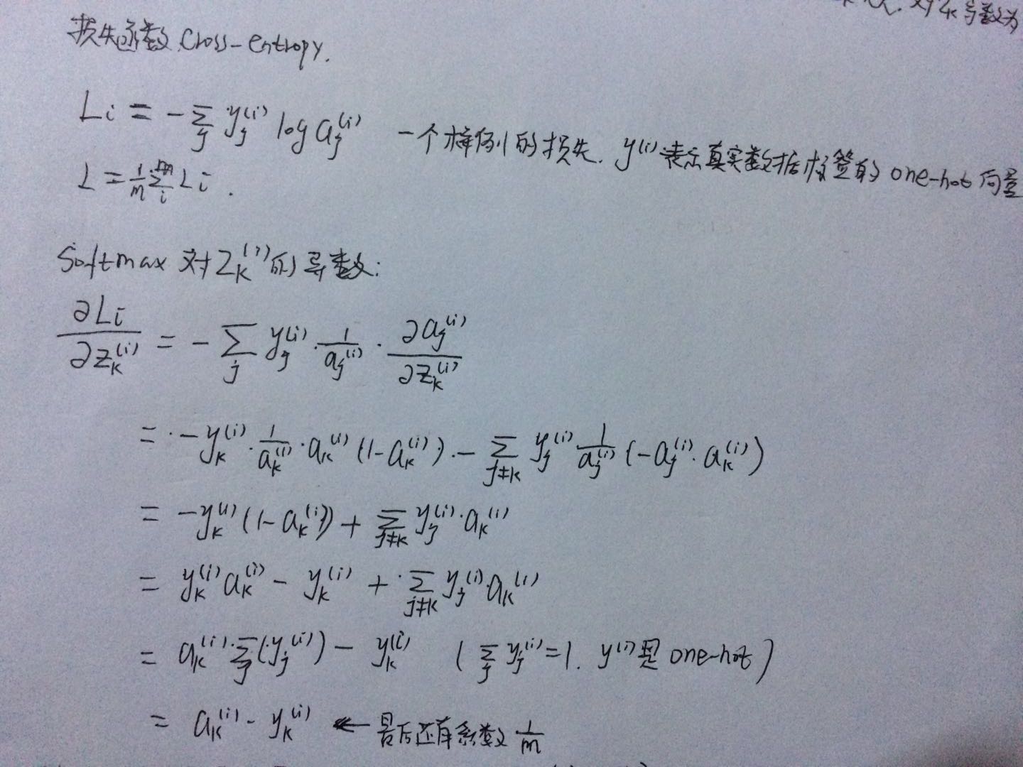
$$
L_i = -\sum_j y^{(i)}_j \log a^{(i)}_j \hspace{0.5in}
$$

$$
L = \sum\limits_{i = 0}^{m} L_i
$$

def cross_entropy(Z,y):
    """
    Z is the output from fully connected layer (num_classes x num_examples)
    y is labels (1 x num_examples)
    """
    m = y.shape[1]
    a = softmax(Z)
    log_likelihood = -np.log(a[y, range(m)])
    loss = np.sum(log_likelihood) / m
    return loss

def cross_entropy_one_hot(Z,Y):
    """
    Z is the output from fully connected layer (num_classes x num_examples)
    Y is labels (nums_classes x num_examples)
    """
    m = Y.shape[1]
    a = softmax(Z)
    log_likelihood = - np.log(a) * Y
    loss = np.sum(log_likelihood) / m
    return loss

3 - softmax derivative

softmax 的求导过程:

softmax 函数对 z 的导数推导

softmax cross entropy loss 对 z 的求导过程:

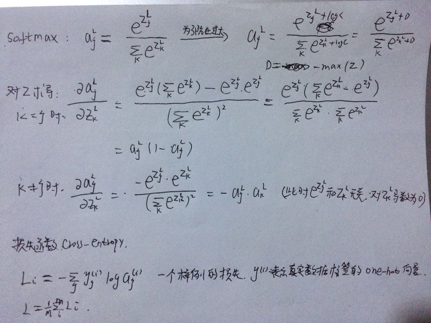
softmax cross entropy loss 对 z 的求导过程

下面是softmax导数的矩阵形式:

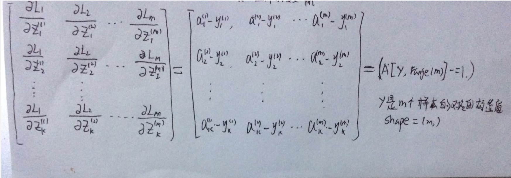
softmax cross-entropy loss derivative matrix

def delta_cross_entropy(Z,y):
    """
    Z is the output from fully connected layer (num_classes x num_examples)
    y is labels (1 x num_examples)
    """
    m = y.shape[1]
    grad = softmax(Z)
    grad[y, range(m)] -= 1
    grad = grad/m
    return grad

def delta_cross_entropy_one_hot(Z,Y):
    """
    Z is the output from fully connected layer (num_classes x num_examples)
    y is labels (num_classes x num_examples)
    """
    m = Y.shape[1]
    grad = softmax(Z)
    grad -= Y
    grad = grad/m
    return grad

参考

深度神经网络(Deep Neural Net)

initialization parameters

1.1 - L-layer Neural Network

The initialization for a deeper L-layer neural network is more complicated because there are many more weight matrices and bias vectors. When completing the initialize_parameters_deep, you should make sure that your dimensions match between each layer. Recall that $n^{[l]}$ is the number of units in layer $l$. Thus for example if the size of our input $X$ is $(12288, 209)$ (with $m=209$ examples) then:

	Shape of W	Shape of b	Activation	Shape of Activation
Layer 1	$(n^{[1]},12288)$	$(n^{[1]},1)$	$Z^{[1]} = W^{[1]} X + b^{[1]} $	$(n^{[1]},209)$
Layer 2	$(n^{[2]}, n^{[1]})$	$(n^{[2]},1)$	$Z^{[2]} = W^{[2]} A^{[1]} + b^{[2]}$	$(n^{[2]}, 209)$
$\vdots$	$\vdots$	$\vdots$	$\vdots$	$\vdots$
Layer L-1	$(n^{[L-1]}, n^{[L-2]})$	$(n^{[L-1]}, 1)$	$Z^{[L-1]} = W^{[L-1]} A^{[L-2]} + b^{[L-1]}$	$(n^{[L-1]}, 209)$
Layer L	$(n^{[L]}, n^{[L-1]})$	$(n^{[L]}, 1)$	$Z^{[L]} = W^{[L]} A^{[L-1]} + b^{[L]}$	$(n^{[L]}, 209)$

Remember that when we compute $W X + b$ in python, it carries out broadcasting. For example, if:

$$ W = \begin{bmatrix}
j & k & l\\
m & n & o \\
p & q & r
\end{bmatrix}\;\;\; X = \begin{bmatrix}
a & b & c\\
d & e & f \\
g & h & i
\end{bmatrix} \;\;\; b =\begin{bmatrix}
s \\
t \\
u
\end{bmatrix}\tag{2}$$

Then $WX + b$ will be:

$$ WX + b = \begin{bmatrix}
(ja + kd + lg) + s & (jb + ke + lh) + s & (jc + kf + li)+ s\\
(ma + nd + og) + t & (mb + ne + oh) + t & (mc + nf + oi) + t\\
(pa + qd + rg) + u & (pb + qe + rh) + u & (pc + qf + ri)+ u
\end{bmatrix}\tag{3} $$

Exercise: Implement initialization for an L-layer Neural Network.

Instructions:
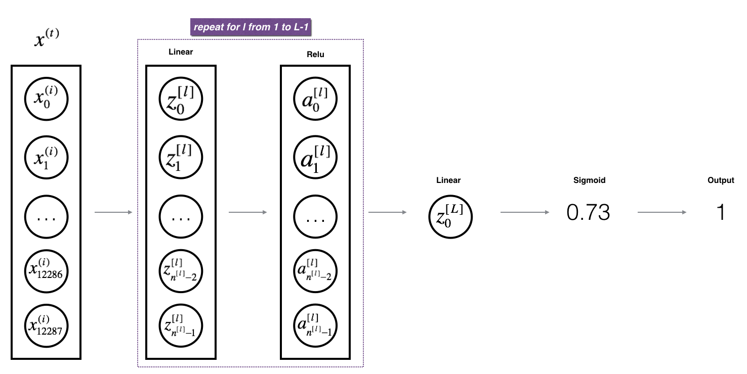
- The model's structure is [LINEAR -> RELU] $ \times$ (L-1) -> LINEAR -> SIGMOID. I.e., it has $L-1$ layers using a ReLU activation function followed by an output layer with a sigmoid activation function.
- Use random initialization for the weight matrices. Use np.random.rand(shape) * 0.01.
- Use zeros initialization for the biases. Use np.zeros(shape).
- We will store $n^{[l]}$, the number of units in different layers, in a variable layer_dims. For example, the layer_dims for the "Planar Data classification model" from last week would have been [2,4,1]: There were two inputs, one hidden layer with 4 hidden units, and an output layer with 1 output unit. Thus means W1's shape was (4,2), b1 was (4,1), W2 was (1,4) and b2 was (1,1). Now you will generalize this to $L$ layers!
- Here is the implementation for $L=1$ (one layer neural network). It should inspire you to implement the general case (L-layer neural network).

    if L == 1:
        parameters["W" + str(L)] = np.random.randn(layer_dims[1], layer_dims[0]) * 0.01
        parameters["b" + str(L)] = np.zeros((layer_dims[1], 1))

# GRADED FUNCTION: initialize_parameters_deep

def initialize_parameters_deep(layer_dims):
    """
    Arguments:
    layer_dims -- python array (list) containing the dimensions of each layer in our network

    Returns:
    parameters -- python dictionary containing your parameters "W1", "b1", ..., "WL", "bL":
                    Wl -- weight matrix of shape (layer_dims[l], layer_dims[l-1])
                    bl -- bias vector of shape (layer_dims[l], 1)
    """

    np.random.seed(3)
    parameters = {}
    L = len(layer_dims)            # number of layers in the network

    for l in range(1, L):
        ### START CODE HERE ### (≈ 2 lines of code)
        parameters['W' + str(l)] = np.random.randn(layer_dims[l], layer_dims[l-1]) * 0.01
        parameters['b' + str(l)] = np.zeros((layer_dims[l], 1))
        ### END CODE HERE ###

        assert(parameters['W' + str(l)].shape == (layer_dims[l], layer_dims[l-1]))
        assert(parameters['b' + str(l)].shape == (layer_dims[l], 1))


    return parameters

4 - Forward propagation module

4.1 - Linear Forward

Now that you have initialized your parameters, you will do the forward propagation module. You will start by implementing some basic functions that you will use later when implementing the model. You will complete three functions in this order:

LINEAR
LINEAR -> ACTIVATION where ACTIVATION will be either ReLU or Sigmoid.
[LINEAR -> RELU] $\times$ (L-1) -> LINEAR -> SIGMOID (whole model)

The linear forward module (vectorized over all the examples) computes the following equations:

$$Z^{[l]} = W^{[l]}A^{[l-1]} +b^{[l]}\tag{4}$$

where $A^{[0]} = X$.

Exercise: Build the linear part of forward propagation.

Reminder:
The mathematical representation of this unit is $Z^{[l]} = W^{[l]}A^{[l-1]} +b^{[l]}$. You may also find np.dot() useful. If your dimensions don't match, printing W.shape may help.

# GRADED FUNCTION: linear_forward

def linear_forward(A, W, b):
    """
    Implement the linear part of a layer's forward propagation.

    Arguments:
    A -- activations from previous layer (or input data): (size of previous layer, number of examples)
    W -- weights matrix: numpy array of shape (size of current layer, size of previous layer)
    b -- bias vector, numpy array of shape (size of the current layer, 1)

    Returns:
    Z -- the input of the activation function, also called pre-activation parameter 
    cache -- a python dictionary containing "A", "W" and "b" ; stored for computing the backward pass efficiently
    """

    ### START CODE HERE ### (≈ 1 line of code)
    Z = np.add(np.dot(W, A), b)
    ### END CODE HERE ###

    assert(Z.shape == (W.shape[0], A.shape[1]))
    cache = (A, W, b)

    return Z, cache

4.2 - Linear-Activation Forward

In this notebook, you will use two activation functions:

Sigmoid: $\sigma(Z) = \sigma(W A + b) = \frac{1}{ 1 + e^{-(W A + b)}}$. We have provided you with the sigmoid function. This function returns two items: the activation value "a" and a "cache" that contains "Z" (it's what we will feed in to the corresponding backward function). To use it you could just call:

A, activation_cache = sigmoid(Z)

ReLU: The mathematical formula for ReLu is $A = RELU(Z) = max(0, Z)$. We have provided you with the relu function. This function returns two items: the activation value "A" and a "cache" that contains "Z" (it's what we will feed in to the corresponding backward function). To use it you could just call:

A, activation_cache = relu(Z)

# GRADED FUNCTION: linear_activation_forward

def linear_activation_forward(A_prev, W, b, activation):
    """
    Implement the forward propagation for the LINEAR->ACTIVATION layer

    Arguments:
    A_prev -- activations from previous layer (or input data): (size of previous layer, number of examples)
    W -- weights matrix: numpy array of shape (size of current layer, size of previous layer)
    b -- bias vector, numpy array of shape (size of the current layer, 1)
    activation -- the activation to be used in this layer, stored as a text string: "sigmoid" or "relu"

    Returns:
    A -- the output of the activation function, also called the post-activation value 
    cache -- a python dictionary containing "linear_cache" and "activation_cache";
             stored for computing the backward pass efficiently
    """

    if activation == "sigmoid":
        # Inputs: "A_prev, W, b". Outputs: "A, activation_cache".
        ### START CODE HERE ### (≈ 2 lines of code)
        Z, linear_cache = linear_forward(A_prev, W, b)
        A, activation_cache = sigmoid(Z)
        ### END CODE HERE ###

    elif activation == "relu":
        # Inputs: "A_prev, W, b". Outputs: "A, activation_cache".
        ### START CODE HERE ### (≈ 2 lines of code)
        Z, linear_cache = linear_forward(A_prev, W, b)
        A, activation_cache = relu(Z)
        ### END CODE HERE ###

    assert (A.shape == (W.shape[0], A_prev.shape[1]))
    cache = (linear_cache, activation_cache)

    return A, cache

d) L-Layer Model

For even more convenience when implementing the $L$-layer Neural Net, you will need a function that replicates the previous one (linear_activation_forward with RELU) $L-1$ times, then follows that with one linear_activation_forward with SIGMOID.

Figure 2 : [LINEAR -> RELU] $\times$ (L-1) -> LINEAR -> SIGMOID model

Exercise: Implement the forward propagation of the above model.

Instruction: In the code below, the variable AL will denote $A^{[L]} = \sigma(Z^{[L]}) = \sigma(W^{[L]} A^{[L-1]} + b^{[L]})$. (This is sometimes also called Yhat, i.e., this is $\hat{Y}$.)

Tips:
- Use the functions you had previously written
- Use a for loop to replicate [LINEAR->RELU] (L-1) times
- Don't forget to keep track of the caches in the "caches" list. To add a new value c to a list, you can use list.append(c).

5 - Cost function

Now you will implement forward and backward propagation. You need to compute the cost, because you want to check if your model is actually learning.

Exercise: Compute the cross-entropy cost $J$, using the following formula: $$-\frac{1}{m} \sum\limits_{i = 1}^{m} (y^{(i)}\log\left(a^{[L] (i)}\right) + (1-y^{(i)})\log\left(1- a^{[L] (i)}\right)) \tag{7}$$

# GRADED FUNCTION: compute_cost

def compute_cost(AL, Y):
    """
    Implement the cost function defined by equation (7).

    Arguments:
    AL -- probability vector corresponding to your label predictions, shape (1, number of examples)
    Y -- true "label" vector (for example: containing 0 if non-cat, 1 if cat), shape (1, number of examples)

    Returns:
    cost -- cross-entropy cost
    """

    m = Y.shape[1]

    # Compute loss from aL and y.
    ### START CODE HERE ### (≈ 1 lines of code)
    cost = - 1. / m * np.sum(Y * np.log(AL) + (1 - Y) * np.log(1 - AL), axis=1, keepdims=True)
    ### END CODE HERE ###

    cost = np.squeeze(cost)      # To make sure your cost's shape is what we expect (e.g. this turns [[17]] into 17).
    assert(cost.shape == ())

    return cost

6 - Backward propagation module

Just like with forward propagation, you will implement helper functions for backpropagation. Remember that back propagation is used to calculate the gradient of the loss function with respect to the parameters.

Reminder:

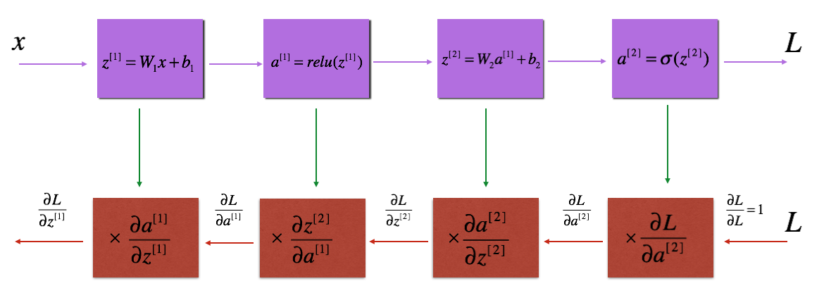
Figure 3 : Forward and Backward propagation for LINEAR->RELU->LINEAR->SIGMOID
The purple blocks represent the forward propagation, and the red blocks represent the backward propagation.

Now, similar to forward propagation, you are going to build the backward propagation in three steps:
- LINEAR backward
- LINEAR -> ACTIVATION backward where ACTIVATION computes the derivative of either the ReLU or sigmoid activation
- [LINEAR -> RELU] $\times$ (L-1) -> LINEAR -> SIGMOID backward (whole model)

6.1 - Linear backward

For layer $l$, the linear part is: $Z^{[l]} = W^{[l]} A^{[l-1]} + b^{[l]}$ (followed by an activation).

Suppose you have already calculated the derivative $dZ^{[l]} = \frac{\partial \mathcal{L} }{\partial Z^{[l]}}$. You want to get $(dW^{[l]}, db^{[l]} dA^{[l-1]})$.

Figure 4

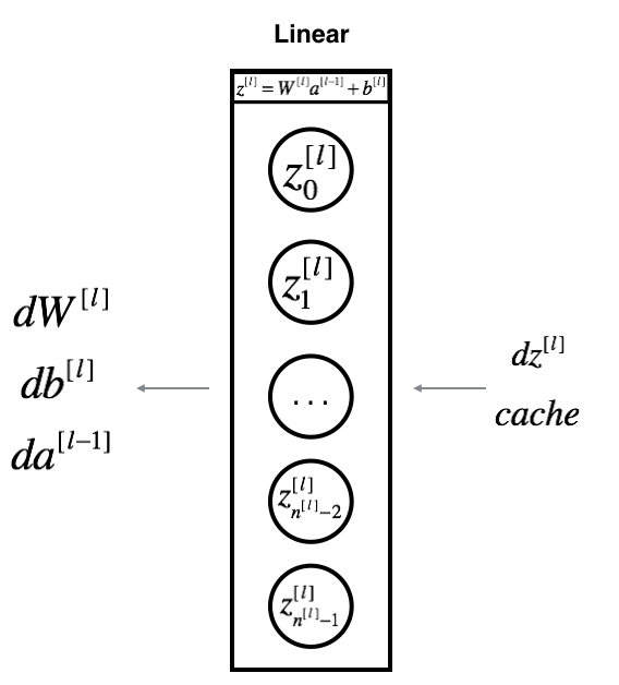
The three outputs $(dW^{[l]}, db^{[l]}, dA^{[l]})$ are computed using the input $dZ^{[l]}$.Here are the formulas you need:
$$ dW^{[l]} = \frac{\partial \mathcal{L} }{\partial W^{[l]}} = \frac{1}{m} dZ^{[l]} A^{[l-1] T} \tag{8}$$
$$ db^{[l]} = \frac{\partial \mathcal{L} }{\partial b^{[l]}} = \frac{1}{m} \sum_{i = 1}^{m} dZ^{[l] (i)}\tag{9}$$
$$ dA^{[l-1]} = \frac{\partial \mathcal{L} }{\partial A^{[l-1]}} = W^{[l] T} dZ^{[l]} \tag{10}$$

# GRADED FUNCTION: linear_backward

def linear_backward(dZ, cache):
    """
    Implement the linear portion of backward propagation for a single layer (layer l)

    Arguments:
    dZ -- Gradient of the cost with respect to the linear output (of current layer l)
    cache -- tuple of values (A_prev, W, b) coming from the forward propagation in the current layer

    Returns:
    dA_prev -- Gradient of the cost with respect to the activation (of the previous layer l-1), same shape as A_prev
    dW -- Gradient of the cost with respect to W (current layer l), same shape as W
    db -- Gradient of the cost with respect to b (current layer l), same shape as b
    """
    A_prev, W, b = cache
    m = A_prev.shape[1]

    ### START CODE HERE ### (≈ 3 lines of code)
    dW = 1. / m * np.dot(dZ, A_prev.T)
    db = 1. / m * np.sum(dZ, axis=1, keepdims=True)
    dA_prev = np.dot(W.T, dZ)
    ### END CODE HERE ###

    assert (dA_prev.shape == A_prev.shape)
    assert (dW.shape == W.shape)
    assert (db.shape == b.shape)

    return dA_prev, dW, db

6.2 - Linear-Activation backward

Next, you will create a function that merges the two helper functions: linear_backward and the backward step for the activation linear_activation_backward.

To help you implement linear_activation_backward, we provided two backward functions:
- sigmoid_backward: Implements the backward propagation for SIGMOID unit. You can call it as follows:

dZ = sigmoid_backward(dA, activation_cache)

relu_backward: Implements the backward propagation for RELU unit. You can call it as follows:

dZ = relu_backward(dA, activation_cache)

If $g(.)$ is the activation function,
sigmoid_backward and relu_backward compute $$dZ^{[l]} = dA^{[l]} * g'(Z^{[l]}) \tag{11}$$.

Exercise: Implement the backpropagation for the LINEAR->ACTIVATION layer.

# GRADED FUNCTION: linear_activation_backward

def linear_activation_backward(dA, cache, activation):
    """
    Implement the backward propagation for the LINEAR->ACTIVATION layer.

    Arguments:
    dA -- post-activation gradient for current layer l 
    cache -- tuple of values (linear_cache, activation_cache) we store for computing backward propagation efficiently
    activation -- the activation to be used in this layer, stored as a text string: "sigmoid" or "relu"

    Returns:
    dA_prev -- Gradient of the cost with respect to the activation (of the previous layer l-1), same shape as A_prev
    dW -- Gradient of the cost with respect to W (current layer l), same shape as W
    db -- Gradient of the cost with respect to b (current layer l), same shape as b
    """
    linear_cache, activation_cache = cache

    if activation == "relu":
        ### START CODE HERE ### (≈ 2 lines of code)
        dZ = relu_backward(dA, activation_cache)
        dA_prev, dW, db = linear_backward(dZ, linear_cache)
        ### END CODE HERE ###

    elif activation == "sigmoid":
        ### START CODE HERE ### (≈ 2 lines of code)
        dZ = sigmoid_backward(dA, activation_cache)
        dA_prev, dW, db = linear_backward(dZ, linear_cache)
        ### END CODE HERE ###

    return dA_prev, dW, db

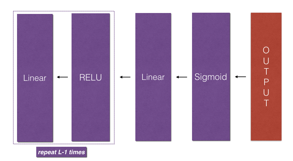
6.3 - L-Model Backward

Now you will implement the backward function for the whole network. Recall that when you implemented the L_model_forward function, at each iteration, you stored a cache which contains (X,W,b, and z). In the back propagation module, you will use those variables to compute the gradients. Therefore, in the L_model_backward function, you will iterate through all the hidden layers backward, starting from layer $L$. On each step, you will use the cached values for layer $l$ to backpropagate through layer $l$. Figure 5 below shows the backward pass.

Figure 5 : Backward pass

Initializing backpropagation:
To backpropagate through this network, we know that the output is,
$A^{[L]} = \sigma(Z^{[L]})$. Your code thus needs to compute dAL $= \frac{\partial \mathcal{L}}{\partial A^{[L]}}$.
To do so, use this formula (derived using calculus which you don't need in-depth knowledge of):

dAL = - (np.divide(Y, AL) - np.divide(1 - Y, 1 - AL)) # derivative of cost with respect to AL

You can then use this post-activation gradient dAL to keep going backward. As seen in Figure 5, you can now feed in dAL into the LINEAR->SIGMOID backward function you implemented (which will use the cached values stored by the L_model_forward function). After that, you will have to use a for loop to iterate through all the other layers using the LINEAR->RELU backward function. You should store each dA, dW, and db in the grads dictionary. To do so, use this formula :

$$grads["dW" + str(l)] = dW^{[l]}\tag{15} $$

For example, for $l=3$ this would store $dW^{[l]}$ in grads["dW3"].

Exercise: Implement backpropagation for the [LINEAR->RELU] $\times$ (L-1) -> LINEAR -> SIGMOID model.

6.4 - Update Parameters

In this section you will update the parameters of the model, using gradient descent:

$$ W^{[l]} = W^{[l]} - \alpha \text{ } dW^{[l]} \tag{16}$$
$$ b^{[l]} = b^{[l]} - \alpha \text{ } db^{[l]} \tag{17}$$

where $\alpha$ is the learning rate. After computing the updated parameters, store them in the parameters dictionary.

Exercise: Implement update_parameters() to update your parameters using gradient descent.

Instructions:
Update parameters using gradient descent on every $W^{[l]}$ and $b^{[l]}$ for $l = 1, 2, ..., L$.

# GRADED FUNCTION: update_parameters

def update_parameters(parameters, grads, learning_rate):
    """
    Update parameters using gradient descent

    Arguments:
    parameters -- python dictionary containing your parameters 
    grads -- python dictionary containing your gradients, output of L_model_backward

    Returns:
    parameters -- python dictionary containing your updated parameters 
                  parameters["W" + str(l)] = ... 
                  parameters["b" + str(l)] = ...
    """

    L = len(parameters) // 2 # number of layers in the neural network

    # Update rule for each parameter. Use a for loop.
    ### START CODE HERE ### (≈ 3 lines of code)
    for l in range(1,L+1):
        parameters["W" + str(l)] = parameters["W" + str(l)] - learning_rate * grads["dW" + str(l)]
        parameters["b" + str(l)] = parameters["b" + str(l)] - learning_rate * grads["db" + str(l)]
    ### END CODE HERE ###
    return parameters